Glossary
A | B | C | D | E | F | G | H | I | J | K | L | M | N | O | P | Q | R | S | T | U | V | W | X | Y | Z
A
| Amplitude | The maximum value over a period of the absolute value of an oscillating function: \(\displaystyle{\max_{t\in[t_0,t_0+T]} \ |f(t)|}\). | The amplitude of \(3\sin(5t)+7\cos(5t) \) does not change: \(\sqrt{3^2+7^2} = \sqrt{58}.\) |
| Autonomous differential equation | A differential equation without terms that depend explicitly on the independent variable. |
\(\dfrac{dP}{dt} = 0.7 P(t) - 20\) Not autonomous: \(\dfrac{dP}{dt} = 0.7 P(t) + 2\sin(t)\) |
| Analytical solution | Exact solution: a formula in closed form. See also Numerical solution. | \(P(t) = 2 e^{0.7t}\) is an analytical solution of \(\dfrac{dP}{dt} = 0.7 P(t)\) |
| Asymptotically stable equilibrium point | A stable equilibrium point, for which, when the initial condition is chosen anywhere in a (small) neighbourhood of the equilibrium point, the solution will tend to the equilibrium point for \(t\rightarrow \infty\). See also: Stable equilibrium point. |
B
| Balance equation | Here: equation that expresses the change in a dependent variable in different constituent terms. | \(\Delta P = b P(t)\Delta t - d P(t) \Delta t\) |
| Birth/Death rate |
The number of population members that are born/die per member of the population per time unit. | \(b = 0.7\) fish per fish per day |
| Boundary conditions (bc) | Fixed conditions for a solution function at different boundaries of the domain. | \(u(0)=0, \ u(10)=1\) |
C
| Center | A stable type of equilibrium point: the matrix of the linearized system in that point has complex eigenvalues with a zero real part ( \(\lambda = \pm \omega i\).) | |
| Coupled differential equations | Systems of differential equations, where at least one of the equation is in more than one dependent variable. |
\(\dfrac{dP}{dt} = 0.7 P(t) - c P(t)\ Y(t)\) \(\dfrac{dY}{dt} = -0.1Y(t)+cP(t)\ Y(t)\) The equations are not coupled when \(c=0\). |
D
| Damped function/solution |
Usually, an oscillating function with period \(T\), of which the amplitude decreases: \(|f(t+T)|<|f(t)|\), for all \(t\). | \(3e^{-0.1t}\sin(5t)\) |
| Derivative | Rate of change of a function: \(\displaystyle{f'(x) = \dfrac{df}{dx} = \lim_{\Delta x \rightarrow 0} \dfrac{f(x+\Delta x) - f(x)}{\Delta x}}.\) | \(\dfrac{d}{dt} e^{kt} = k e^{kt}\) |
| Difference equation |
An equation in the values of a sequence. | \(y_{n+1} = 0.2 y_n + 1\) |
| Difference quotient |
Ratio of the change in a dependent variable and the change in its independent variable: \(\dfrac{\Delta f}{\Delta x} = \dfrac{f(x+\Delta x) - f(x)}{\Delta x}.\) | \(\dfrac{P(t+\Delta t) - P(t)}{\Delta t}\) |
| Differential equation | An equation with derivatives of a function. | \(\dfrac{dP}{dt} = 0.7 P(t)\) |
| Direction field | Graph with small arrows indicating the directions of solutions of differential equations. |
Direction field plus some solution curves. |

E
| Equilibrium point |
Point in which the derivatives of all dependent variables with respect to the independent variable are equal to 0. If an equilibrium point is chosen as initial value, the solution is constant. |
\(\dfrac{dP}{dt} = 0.7 P - P\ Y\) \(\dfrac{dY}{dt} = -0.1Y+PY\) Equilibrium points are \( (0,0) \) and \((10, 0.7)\) |
| Euler's method |
Algorithm to approximate the solution of first-order differential equations. |
for \(\dfrac{dy}{dt} = f(t,y(t))\): \(y((n+1)\Delta t) \approx y(n\Delta t) + \Delta t f(n\Delta t, y(n\Delta t) \) |
F
G
| General solution of a differential equation |
Function that fulfills the differential equation. The function contains one or more free constants: no initial conditions have been applied yet. | \(P(t) = c_1 e^{0.7t}\) is the general solution of \(\dfrac{dP}{dt} = 0.7P(t)\) |
| Gourami | A group of freshwater fishes, e.g. paradise gouramis | 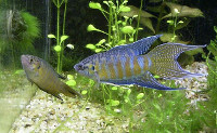 |
H
| Homogeneous differential equation |
Differential equation in which all terma depend on the dependent variable. See also: Inhomogeneous differential equation | \(\dfrac{dP}{dt} = 0.7 P(t)\) |
I
| Independent/Dependent variables |
When \(f\) is a function of variable \(x\), so \(f=f(x)\), then \(x\) is the independent variable, and \(f\) the dependent variable. | Time \(t\) is an independent variable. \(P(t)\) is a dependent variable. |
| Inhomogeneous differential equation |
A differential equation that contains a term without the dependent variable (usually representing an external influence). See also Homogeneous differential equation |
\(\dfrac{dP}{dt} = 0.7 P(t)+20\sin(t)\) |
| Initial condition (ic) |
The value of a dependent variable or one of its derivatives at the initial time (often \(t=0\)). | \(P(0)=30\) |
| Integrating a differential equation |
Solving a differential equation, usually analytically. |
J
K
L
| \(\LaTeX\) | A document preparation system used for technical and scientific texts. | |
| Logistic function | A solution of a differential equation with logistic growth. The graph of the solution is shaped like a stretched letter S. |  |
M
| Mathematical model |
A representation of a real-life phenomenon in mathematical formulas | \(\dfrac{dP}{dt} = 0.7P(t), \ P(0)=20\) |
| Modified Euler Method |
Another numerical integration method. See also: Euler's method |
N
| Node | A type of equilibrium point: the matrix of the linearized system in that point has only real eigenvalues that are either all positive (an unstable node), or all negative (a stable node). | |
| Numerical approximation | An approximate solution obtained using an approximate (computer) algorithm. See also: Analytical solution |
O
| Order of a differential equation |
The highest order of a derivative in a differential equation. | The order of \(u''+u=f(t)\) is two. |
| Ordinary differential equation (ode) |
A differential equation with only ordinary derivatives; there is only one independent variable. See also: Partial differential equation |
\(\dfrac{dP}{dt} = 0.7P(t)\) |
| Oscillating solution |
The solution is alternatingly increasing and decreasing. | \(3e^{-0.1t}\sin(5t)\) |
P
| Partial differential equation (pde) |
A differential equation with partial derivatives; there are at least two independent variables. See also: Ordinary differential equation |
\(\alpha^2 \dfrac{\partial^2 u(x,t)}{\partial x^2} = \dfrac{\partial u(x,t)}{\partial t} \) |
| Periodic function |
A function \(f(t)\) is periodic, with period \(T\) when \(f(t+T) = f(t).\) | \(\sin(15t)\) is a periodic function with period \(T=\dfrac{2\pi}{15}.\) |
| Phase line |
(Graph of) a line (segment) representing values of a dependent variable, usually with equilibrium points and arrows indicating the direction of the evolution of the variable. |  |
| Phase plane |
Plane of points \((x(t),y(t))\) where \(x(t)\) and \(y(t)\) are both dependent variables (of the same independent variable, here \(t\) ). | |
| Phase space |
\(n\)-dimensional space of points \((x_1(t), x_2(t), \ldots,x_n(t))\), with \(n\ge3\). | |
| Python | A programming language for general-purpose programming |
Q
R
| Rainbowfish | Family of small, colourful, freshwater fish found in Australia, New Guinea and Indonesia. | 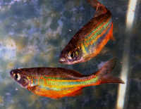 |
| Runge-Kutta method |
Family of numerical integration methods. See also: Euler's Method |
S
| Saddle point |
A type of equilibrium point: the matrix of the linearized system in that point has only real eigenvalues of which at least one is positive, and another one is negative. A saddle point is an unstable equilibrium point. | |
| Slope field |
See: Direction field | |
| Solving a differential equation |
Finding a function that fulfills the differential equation (analytically). | \(P(t)=2e^{0.7t}\) is a solution of \(\dfrac{dP}{dt}=0.7P(t).\) |
| Spiral point |
A type of equilibrium point: the matrix of the linearized system in that point has complex eigenvalues \(\lambda = a \pm \omega i\) with \(\omega \ne 0\). If \(a>0\) the spiral point is unstable, if \(a<0\) the spiral point is stable. | |
| Stable equilibrium point |
If the initial condition is chosen anywhere in a (small) neighbourhood of the equilibrium point, the solution will remain close to that equilibrium point for all times. See also: Unstable equilibrium point, Asymptotically stable equilibrium point. | |
| Stable node |
A type of equilibrium point: the matrix of the linearized system in that point has only real eigenvalues that are all negative. See also: Unstable node. |
|
| Stable numerical method |
In a numerical integration method, an error is made in each step. In the next step(s), the result of the earlier step is used, including the error. A numerical method is stable for a specific problem and stepsize, if the error made in one of the steps is not transferred to the following step with an increased size. See also: Unstable numerical method. | |
| Stable spiral point |
A type of equilibrium point: the matrix of the linearized system in that point has complex eigenvalues \(\lambda = a \pm \omega i\), where \(\omega \ne 0\) and where \(a < 0\). See also: Unstable spiral point. |
|
| Stationary point |
See: Equilibrium point. | |
| Stepsize | The length of the steps in the independent variable in a numerical method. | \(\Delta t\) |
T
| Tangent line |
Linearisation of a function of one variable. The line tangent to function \(f(x)\) in point \(x=a\) with the equation: \(L(x) = f(a) + \dfrac{df(a)}{dx} (x-a)\). | The line tangent to \(f(x)=x^2\) in \(x=3\): \(L(x) = 9+6(x-3)\) |
| Tangent plane |
Linearisation of a function of more than one variables. The tangent plane to function \(f(x,y)\) in point \((x,y)=(a,b)\) has the equation: \(L(x,y) = f(a,b) + \dfrac{\partial f(a,b)}{\partial x} \ (x-a) + \dfrac{\partial f(a,b)}{\partial y}.\) | The plane tangent to \(f(x,y)=x^2\sin(3y)\) in \((x,y)=(3,\dfrac{\pi}{9})\): \(L(x,y) = \) \(\dfrac{9\sqrt{3}}{2}+3\sqrt{3}(x-3) \) \(+ \dfrac{27}{2}(y-\dfrac{\pi}{9})\) |
U
| Unstable equilibrium point |
Any equilibrium point that is not stable. There is at least one initial condition in a (small) neighbourhood of the equilibrium point, for which the the solution will not remain close to that equilibrium point for all times. See also: Stable equilibrium point. | |
| Unstable node |
A type of equilibrium point: the matrix of the linearized system in that point has only real eigenvalues that are all positive. See also: Stable node. | |
| Unstable numerical method |
In a numerical integration method, an error is made in each step. In the next step(s), the result of the earlier step is used, including the error. A numerical method is unstable for a specific problem and stepsize, if the error made in one of the steps might be transferred to the following step with an increased size. See also: Stable numerical method. | |
| Unstable spiral point |
A type of equilibrium point: the matrix of the linearized system in that point has complex eigenvalues \(\lambda = a \pm \omega i\), where \(\omega \ne 0\) and where \(a > 0\). See also: Stable spiral point. |